A signal can contain multiple periodic functions with different amplitudes and frequencies. The Fourier Transform is able to decompose a signal down into the individual sine functions that constitute the overall signal.
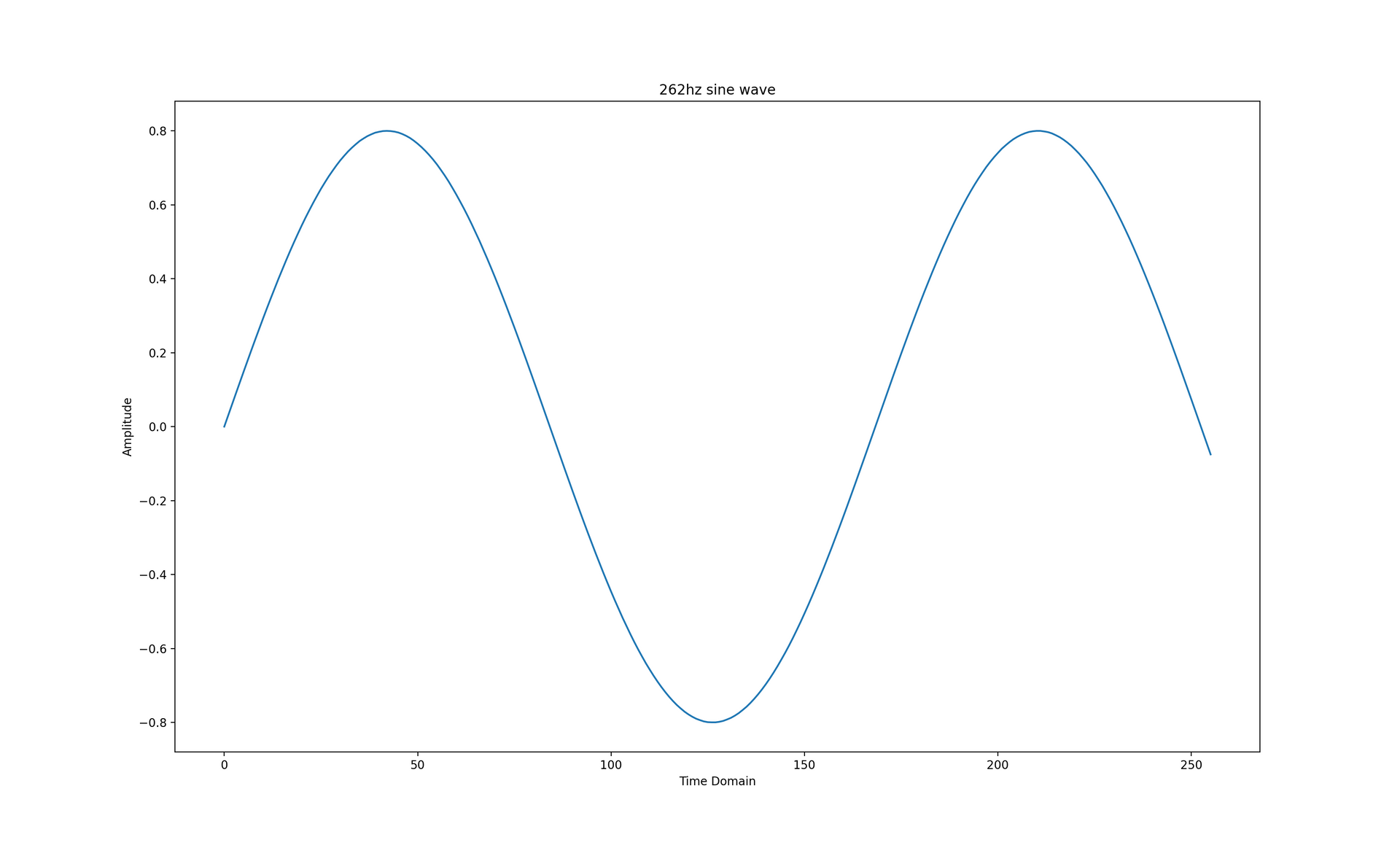
Let's say your signal is a 262hz (or middle C) sine wave, encoded as a Pulse Code Modulation (PCM) stream with a sample rate of 44100 samples per second. According to the Nyquist–Shannon sampling theorem, a signal can represent a frequency range of half of the sampling rate. A PCM sample rate of 44100 samples per second translates to a frequency range between 0-22050hz.
A DFT configured with a window size of 256 means it will operate on a block of 256 chronologically ordered signal samples. The maximum resolution of the DFT is dictated by the window size and the frequency range of the input signal. This DFT operating on the PCM signal from the previous paragraph would have a resolution of \(\frac{44100}{256} = 172.266hz\) and would detect a dominant frequency range between 172.266hz and 344.531hz.
The Discrete Fourier Transform (DFT) is defined by the following equation.
\begin{equation}
X_{k} = \sum_{n=0}^N x_{n} e^{\frac{-2 i \pi n k}{N}}
\end{equation}
\(X_{k}\) represents the fourier transform for frequency bin \(k\), where \(0 \le k \le N\) and each transform for k represents a slice of the frequency spectrum from \(k \cdot \frac{y}{N}\) to \(k \cdot \frac{y}{N} + \frac{y}{N}\), where \(y\) represents the original sample rate of the signal and \(N\) represents the window size of the DFT.
n.b. Raising e to an imaginary number represents Euler's formula, i.e. \(e^{ix} = cos(x) - isin(x)\). If using a language without built-in complex number support, you would calculate the real and imaginary components separately by passing \(\frac{-2 \pi n k}{N}\) into the cosine and sine functions, respectively. Complex numbers are denoted by the letter j in Python, so np.exp(1j * np.pi) is the same as cos(π) - isin(π).
Surfing On Sine Waves
The code below generates a 262hz sine wave represented as a 1 second long, 16-bit floating point PCM stream with a sample rate of 44100 samples per second. The generated graph only shows the time domain of the signal from 0 up to windows_size because this is the signal subset the subsequent Discrete Fourier Transforms will operate on. All of the subsequent code samples depend on this one.
from matplotlib import pyplot as plt
import pandas as pd
import numpy as np

window_size = 256 # Experiment with this value, it should always be a power of two.
sample_rate = 44100
frequency = 262
seconds = 1
sample_count = sample_rate * seconds
pcm_stream_16bit = list(map(lambda x : np.float16(0.8 * np.sin(2.0 * np.pi *
frequency * x / sample_rate)), np.arange(sample_count)))
s = pd.Series(pcm_stream_16bit[:window_size], index=np.arange(sample_count)[:window_size])

s.plot.line(figsize=(20,10))
plt.xlabel('Time Domain')
plt.ylabel('Amplitude')
plt.title(f'{frequency}hz sine wave')
plt.show()

step = sample_rate / window_size
print(f'Minimum unit size: {step}hz\n')

pcm = pcm_stream_16bit[:window_size]
pivot = len(pcm) // 2

Brute Force
The next code snippet demonstrates how a brute force DFT on samples 0 to window_size from the PCM stream works. It outputs the sum of each frequency bin and determines which one is dominant. The outer loop has one iteration for each frequency bin / k-bin, the inner loop has one iteration for each PCM sample.
As you can see from the code, we only care about the first half of the DFT for figuring out the dominant frequency because when the DFT input is a sequence of real numbers (instead of complex), the output will have conjugate symmetry. In practical terms, the real valued DFT output mirrors the first half of the output sequence in the second half.
import numpy as np

column_width = 45
pcm_column_width = 20

iterations = 0
largest = 0j
largest_index = 0

for k in range(0, len(pcm)):
    frequency_bin = [0j] * len(pcm)
    for i in range(0, len(pcm)):
        exponent = np.exp(-2.0j * np.pi * i * k / len(pcm))
        result = pcm[i] * exponent
        iterations = iterations + 1
        frequency_bin[i] = frequency_bin[i] + result

    total = sum(frequency_bin)
    print(f'TOTAL (FREQUENCY BIN / K-BIN {k}): {total}')

    # We only care about the first half of the DFT because
    # of Conjugate symmetry, as explained earlier.
    if total > largest and k < len(pcm) // 2:
        largest = total
        largest_index = k

print(f'\nMinimum unit size: {step}hz\n')
print(f'Iterations: {iterations}')
print(f'Largest: {largest} {largest_index}')
print(f'hz: {largest_index * step} - {(largest_index * step) + step}')
Perfect Specimen
Numpy provides a production level Fast Fourier Transform (FFT), it's a good point of reference.
print(list(np.fft.fft(pcm, len(pcm))))
The outputted values are virtually the same, although rounding can make them appear less alike than they really are. The specifics of rounding complex floating point numbers are a rabbit hole for another day! If you doubt what I'm saying, stick the outputs on a graph.
Cooley-Tukey For Programmers
I'm going to walk through how the Cooley-Tukey FFT equation is derived from the DFT equation (shown earlier) using code examples to provide a sort of "inductive walkthrough for programmers". Each snippet depends on the first code snippet and I'd recommend running them all locally and comparing them to get the most from this guide.
The DFT can be calculated from the sum of two smaller DFTs. If you perform a DFT on the even and odd parts of the input, for example, you end up doing two \(\frac{N}{2}\) sized FFTs.
\begin{equation}
X_{k} = \sum_{n=0}^N x_{n} e^{\frac{-2 i \pi n k}{N}} = \sum_{n=0}^{N/2} x_{2 n} e^{\frac{-2 i \pi (2 n) k}{N}} + \sum_{n=0}^{N/2} x_{2 n + 1} e^{\frac{-2 i \pi (2 n + 1) k}{N}}
\end{equation}
The code below demonstrates that the equality relationship in the above formula is true.
iterations = 0
transform_vector = [0j] * len(pcm)
for k in range(0, len(pcm)):
    for m in range(0, pivot):
        iterations = iterations + 1
        transform_vector[k] = transform_vector[k] + (pcm[2 * m] * np.exp(-2j * np.pi * (2 * m) * k / len(pcm)))

for k in range(0, len(pcm)):
    for m in range(0, pivot):
        iterations = iterations + 1
        transform_vector[k] = transform_vector[k] + (pcm[2 * m + 1] * np.exp(-2j * np.pi * (2 * m + 1) * k / len(pcm)))

print(f'Iterations: {iterations}\n')
print(list(transform_vector))
The even and odd side of the equation are almost identical, the only difference is that the odd DFT exponent has \(2n + 1\) instead of \(2n\). If we could make both exponents identical, we would be able to calcualte \(e^{\frac{-2 \pi i (2 n) k}{N}}\) once for both sides of the equation.
Fortunately, all we have to do is factor a common multiplier out of the odd side of the equation.
\begin{equation}
X_{k} = \sum_{n=0}^{N/2} x_{2 n} e^{\frac{-2 i \pi n k}{N/2}} + e^{\frac{-2 i \pi k}{N}} \sum_{n=0}^{N/2} x_{2 n + 1} e^{\frac{-2 i \pi n k}{N/2}}
\end{equation}
The odd DFT can now reuse the exponent from the even DFT, we just have to multiply it by the common multiplier. The rearranged formula reduces the total number of calculations required for the full DFT and the number of iterations is also easier to reduce from \(N^2\) to \(\frac{N^2}{2}\). The order of complexity is still \(O(N^2)\).
The code below implements the rearranged equation.
iterations = 0
even_transform_vector = [0j] * len(pcm)
odd_transform_vector = [0j] * len(pcm)
for k in range(0, len(pcm)):
    for m in range(0, pivot):
        iterations = iterations + 1
        e = np.exp(-2j * np.pi * m * k / pivot)
        even_transform_vector[k] = even_transform_vector[k] + (pcm[2 * m] * e)
        odd_transform_vector[k] = odd_transform_vector[k] + (pcm[2 * m + 1] * e)
    odd_transform_vector[k] = odd_transform_vector[k] * np.exp(-2j * np.pi * k / len(pcm))

print(f'Iterations: {iterations}\n')
print(list(np.add(even_transform_vector, odd_transform_vector)))
We can calculate \(X_{k+\frac{N}{2}}\) using the equation for \(X_{k}\) if we add \(\frac{N}{2}\) to \(k\).
\begin{equation}
X_{k+\frac{N}{2}} = \sum_{n=0}^{N/2} x_{2 n} e^{\frac{-2 i \pi n (k+\frac{N}{2})}{N/2}} + e^{\frac{-2 i \pi (k+\frac{N}{2})}{N}} \sum_{n=0}^{N/2} x_{2 n + 1} e^{\frac{-2 i \pi n (k+\frac{N}{2})}{N/2}}
\end{equation}
This can halve the number of iterations of the k-loop because we can calculate \(X_{k+\frac{N}{2}}\) while we're calculating \(X_{k}\)
The implementation below demonstrates that the iteration count is a quarter of what is was in the previous step.
iterations = 0
even_transform_vector = [0j] * len(pcm)
odd_transform_vector = [0j] * len(pcm)
for k in range(0, pivot):
    for m in range(0, pivot):
        iterations = iterations + 1

        # X(k)
        e = np.exp(-2j * np.pi * m * k / pivot)
        even_transform_vector[k] = even_transform_vector[k] + (pcm[2 * m] * e)
        odd_transform_vector[k] = odd_transform_vector[k] + (pcm[2 * m + 1] * e)

        # X(k + N/2)
        e = np.exp(-2j * np.pi * m * (k + pivot) / pivot)
        even_transform_vector[k + pivot] = even_transform_vector[k + pivot] + (pcm[2 * m] * e)
        odd_transform_vector[k + pivot] = odd_transform_vector[k + pivot] + (pcm[2 * m + 1] * e)

    # X(k)
    odd_transform_vector[k] = odd_transform_vector[k] * np.exp(-2j * np.pi * k / len(pcm))

    # X(k + N/2)
    odd_transform_vector[k + pivot] = odd_transform_vector[k + pivot] * np.exp(-2j * np.pi * (k + pivot) / len(pcm))

print(f'Iterations: {iterations}\n')
print(list(np.add(even_transform_vector, odd_transform_vector)))
The only real difference between \(X_{k}\) and \(X_{k+\frac{N}{2}}\) is that the latter adds \(\frac{N}{2}\) to k. If we could make them more alike, we could calculate one exponent and use it twice.
Fortunately, we can factor \(\frac{N}{2}\) out of the \(k+\frac{N}{2}\) side by applying the common multiplier, \(e^{-2 \pi i m}\).
\begin{equation}
X_{k+\frac{N}{2}} = \sum_{n=0}^{N/2} x_{2 n} e^{\frac{-2i \pi n k}{N/2}} e^{-2i \pi m} +
e^{\frac{-2 i \pi k}{N}} e^{-\pi i} \sum_{n=0}^{N/2} x_{2 n + 1} e^{\frac{-2 i \pi n k}{N/2}} e^{-2i \pi m}
\end{equation}
The code snippet below demonstrates an implementation of the rearranged equation.
iterations = 0
even_transform_vector = [0j] * len(pcm)
odd_transform_vector = [0j] * len(pcm)
for k in range(0, pivot):
    for m in range(0, pivot):
        iterations = iterations + 1

        # X(k)
        e1 = np.exp(-2j * np.pi * m * k / pivot)
        even_transform_vector[k] = even_transform_vector[k] + (pcm[2 * m] * e1)
        odd_transform_vector[k] = odd_transform_vector[k] + (pcm[2 * m + 1] * e1)

        # X(k + N/2)
        e2 = e1 * np.exp(-2j * np.pi * m)
        even_transform_vector[k + pivot] = even_transform_vector[k + pivot] + (pcm[2 * m] * e2)
        odd_transform_vector[k + pivot] = odd_transform_vector[k + pivot] + (pcm[2 * m + 1] * e2)

    # X(k)
    e3 = np.exp(-2j * np.pi * k / len(pcm))
    odd_transform_vector[k] = odd_transform_vector[k] * e3

    # X(k + N/2)
    e4 = e3 * np.exp(np.pi * 1j)
    odd_transform_vector[k + pivot] = odd_transform_vector[k + pivot] * e4

print(f'Iterations: {iterations}\n')
print(list(np.add(even_transform_vector, odd_transform_vector)))
The snippet below demonstrates why \(e^{\frac{-2i \pi n k}{N/2}} e^{-2i \pi m}\) could be replaced by \(e^{\frac{-2i \pi n k}{N/2}}\).
sum_one = 0j
sum_two = 0j
for k in range(0, len(pcm)):
    for n in range(0, len(pcm)):
        sum_one = sum_one + np.exp(-2j * np.pi * n * k / pivot)
        sum_two = sum_two + np.exp(-2j * np.pi * n * k / pivot) * np.exp(-2j * np.pi * n)

print(round(sum_one, 10))
print(round(sum_two, 10))
print(round(sum_two - sum_one, 10))
So, based on this, we can simply the equation further like so.
\begin{equation}
X_{k+\frac{N}{2}} = \sum_{n=0}^{N/2} x_{2 n} e^{\frac{-2i \pi n k}{N/2}} +
e^{\frac{-2 i \pi k}{N}} e^{-\pi i} \sum_{n=0}^{N/2} x_{2 n + 1} e^{\frac{-2 i \pi n k}{N/2}}
\end{equation}
The snippet below demonstrates why \(e^{\frac{-2i \pi k}{N}} e^{-\pi i}\) could be replaced by \(-e^{\frac{-2i \pi n k}{N}}\)
sum_one = 0j
sum_two = 0j
for k in range(0, pivot):
    sum_one = sum_one + np.exp(-2j * np.pi * k / len(pcm))
    sum_two = sum_two - np.exp(-2j * np.pi * k / len(pcm)) * np.exp(-1j * np.pi)

print(sum_one)
print(sum_two)
The final equation is as follows and it essentially describes the butterfly operation for recombining the sub-transforms.
\begin{equation}
X_{k+\frac{N}{2}} = \sum_{n=0}^{N/2} x_{2 n} e^{\frac{-2i \pi n k}{N/2}} -
e^{\frac{-2 i \pi k}{N}} \sum_{n=0}^{N/2} x_{2 n + 1} e^{\frac{-2 i \pi n k}{N/2}}
\end{equation}
The code below demonstrates the basic (poor performance) idea of the above equation. The code snippet after it is a recursive implementation with an order of complexity of \(O(n log(n)\)
iterations = 0
even_transform_vector = [0j] * len(pcm)
odd_transform_vector = [0j] * len(pcm)
for k in range(0, pivot):
    for m in range(0, pivot):
        iterations = iterations + 1

        # X(k)
        e1 = np.exp(-2j * np.pi * m * k / pivot)
        even_transform_vector[k] = even_transform_vector[k] + (pcm[2 * m] * e1)
        odd_transform_vector[k] = odd_transform_vector[k] + (pcm[2 * m + 1] * e1)


transform = [0j] * len(pcm)
for k in range(0, pivot):
    iterations = iterations + 1
    e = np.exp(-2j * np.pi * k / len(pcm))
    transform[k] = even_transform_vector[k] + e * odd_transform_vector[k]
    transform[k + pivot] = even_transform_vector[k] - e * odd_transform_vector[k]


print(f'Iterations: {iterations}\n')
print(list(transform))
def fft(sample_set):
  if len(sample_set) == 1:
    return sample_set

  size = len(sample_set)
  even_fft = fft(sample_set[0::2])
  odd_fft = fft(sample_set[1::2])

  freq_bins = [0.0] * size
  for k in range(0, int(size / 2)):
    freq_bins[k] = even_fft[k]
    freq_bins[k + int(size / 2)] = odd_fft[k]

  for k in range(0, int(size / 2)):
    e = np.exp(-2j * np.pi * k / size)
    t = freq_bins[k]
    freq_bins[k] = t + e * freq_bins[k + int(size / 2)]
    freq_bins[k + int(size / 2)] = t - e * freq_bins[k + int(size / 2)]

  return freq_bins

print(fft(pcm))
Extra Resources
Here's a list of resources that might help you get unstuck if some my post is unclear. Some of the resources are much more in depth and I'm still learning a lot from them.
Interactive Guide To The Fourier Transform
Fourier Series Intro
Cooley-Tukey Fast Fourier Transform
Butterfly diagram
Fourier Analysis by Georgi P. Tolstov
Nyquist-Shannon Sampling Theorem
Pulse Code Modulation
Euler's Formula
Complex Number Intro
Introduction to Imaginary Numbers
De Moivre Formula
Further Reading
I've implemented a recursive Cooley-Tukey Radix-2 DIT in Python, the script also performs a brute force DFT and a Numpy FFT for comparison.